
A Logit and some elasticities
05 August 13. [link] PDF version
This is a series of posts about doing interesting things with the Apophenia library of stats functions for C. Today's subject will be an analysis of a recent congressional vote regarding the funding of an NSA wiretap program. I'd promised to do this via a Logit. This continues a thread from two entries ago, when I set up Fisher's Exact test to easily reject the hypothesis that two categorical variables (vote, party) are independent. Those of you who are just interested in the results are encouraged to skim or skip the discussions of how the code was assembled. Also, please note that there's a PDF version of this linked above if the math doesn't render right in your browser.
This time, we'll look at contributions from defense contractors (and I will again send you to the blog of Govtrack's proprietor, Josh Tauberer, for details about the variables and their derivations). The short version of the story is that this was a vote to defund an NSA wiretapping program. An Aye vote is thus a vote against the NSA's wiretapping program; a No vote is in support of the wiretapping status quo. To give us one less level of indirection, I'll refer to the votes as anti-tap and pro-tap (and will ignore any quibbling about whether maintaining the status quo is really pro).
Mr Tauberer's entry is in reply to a post in a Condé Nast blog claiming that defense dollars are a better predictor of this vote than ideology. Josh's blog did a fine job of getting across that neither is a stellar predictor, and calls it a draw. I'm not going to revise that here, but will talk about what the Logit says about the effect of ideology and dollars.
Nothing in this discussion will be a slam dunk, but here are some results given the model, before I get into computing technique:
- In aggregate, contributions had a greater influence in pushing the voters toward the pro-tap vote. Reading that the other way, ideology had a greater influence in pulling voters toward a no-tap vote. This is in aggregate; for a minority of observations it goes the other way.
- The blogger for Condé Nast pointed out that the Aye votes received an average of twice the defense money that the No votes received. I verify that this is true below, but that doesn't mean that there's twice the influence.
- In the context of only this vote and this model, a lot of campaign contributions were wasted: the marginal effect of the last dollar in campaign contributions on the vote was frequently almost nil.
The outcome variable is a binary variable (Aye vote or No vote), so we will use a Logit or a Probit. Custom leans toward the Logit, and we'll see the sort of closed-form results we can get out of it below. You can change the apop_logit to apop_probit in the example and see how things change if so desired.
Both the Logit and Probit are generalized linear models. In this case, we contend that
$$P(\textrm{pro-tap}) = \beta_0 + \beta_1 \cdot \textrm{ideology} + \beta_2 \cdot \textrm{defense contributions} + \epsilon.$$
For a Logit, $\epsilon$ has a Gumbel Type II distribution. What's the narrative that would cause errors to have that distribution? Nobody cares; it makes the math easy. At least a Probit has $\epsilon \sim$ Normal.
Coding up the model
This is the first part where some of you will skip to the next section header.
A regression with Apophenia is two steps: data prep, and model estimation. Broadly, I recommend that data prep happen via SQL, which is a data manipulation language entirely built around selecting just the right table from a data set. E.g.,
apop_data *d = apop_query_to_mixed_data("tmm", "select vote, 0, contrib from amash_vote_analysis");
The usual apop_query_to_data function puts all data in the numeric matrix portion of a data set; the apop_query_to_mixed_data function requires that you specify whether each given column is text, numeric, row name, vector, or weight; in this case "tmm" indicates text, matrix, matrix. The point of my exposition last time was to explain why the function requires that you as a human specify these things. The short version: I've never had a system that auto-guessed column types that did not at some point screw me over. However, it is on the to-do list to improve the interface a little.
OK, we have now reliably read the data into an in-memory data set, including both numeric and text elements. Next step: create factors (i.e., numeric representations of categories represented by text data). Although R's automatic factor generation makes things smooth for interactive do-what-I-mean regressions, I have heard too many sob stories from users who were wrestling for control of autogenerated factors. Apophenia requires that we explicitly call apop_data_to_factors in the program below. Unless specified otherwise, the numeric version of the data gets written to column zero of the data, which is why the query set up that column of zeros, reserving space for the factorized votes. We could have obviated all of this by writing the query differently, by the way, but I wanted to demonstrate this stuff. Yet again, a lot of stats packages will produce virtual columns of data that never exist on the hard drive, instead of being so mechanical and literal. There'll be some payoff to the plodding and literal approach below.
Once the data is set up, it's just a question of calling apop_estimate with the data and the model. Here's the full program:
#include

int main(){
    apop_text_to_db("amash_vote_analysis.csv");
    apop_data *d = apop_query_to_mixed_data("mmt", "select 0, ideology, contribs, vote from amash_vote_analysis");
    apop_data_to_factors(d);
    apop_model_show(apop_estimate(d, apop_logit));
}
If you want to try this in R, here's the script. Instead of the four lines of code it took in Apophenia (plus the #include and int main() headers), you can do it in two, because R, like most stats packages, merges the selection of data columns into the model estimation step and we're OK with having Aye=0 in this case, so the autogenerated factors work fine.
d  <- read.csv("amash_vote_analysis.csv")
glm(vote ~ ideology + contribs, data=d, family="binomial")
The output, from both R and C, is a list of coefficients. The relevant ones are 1.64 and 0.000017. It's clearly meaningless to compare them because the scales and units are entirely different, so we need to do some further work to produce something interpretable.
One thing we can say is that both coefficients are positive, so a higher ideology score and higher campaign contributions both lead to higher odds of voting pro-tap.
Using the model results
To give you a metaphor, let's say that we have this equation
$$\textrm{fruits} = \textrm{apples} + \textrm{oranges}.$$
Jane has 4 fruits = 1 apple + 3 oranges; Janet has 8 fruits = 5 apples + 3 oranges. We might be inclined to say that Jane has fewer fruits because she has fewer apples, or that Janet has many fruits because she has more apples. There isn't any true causality here: the fruits simply are. But because the left-hand side of Jane's equation is small, we look for the smaller part of the right-hand side to explain her paucity of fruit; because Janet's left-hand side is large, we look for the larger part of the right-hand side to explain her surplus.
And what about Janice, who has 50 fruits = 5 apples and 45 oranges? If we take the mean of the apple and orange count across everybody, there's clearly a huge surplus of oranges, but if Janice isn't sharing, the orange surplus means nothing to Janet and Jane. Perhaps we're better off taking a per-person tally of whether each person has more oranges or apples.
One nice way to do this is to scale every fruit count to one:
Jane   .25a  to .75o
Janet  .625a to .375o
Janice .1a   to .9o
It's clear that two out of three fruit baskets favor oranges. One could easily construct examples where the mean ratio favors apples but the mean count favors oranges.
So normalizing to one gives us a slightly different analysis than the not-normalized version. I'm going to do the normalized version here, thus focusing on how many congresspeople care about one input over another, and leave the un-normalized version (which is more easily swayed by extreme observations in campaign contribution measures) as an exercise for the reader.
As above, the model takes the form
$$P(\textrm{pro-tap}) = f(\beta_0 + \beta_1 \textrm{ideology} + \beta_2 \textrm{defense contributions}) + \epsilon,$$ and we like that neat linear form because it claims that we can directly compare $\beta_1 \cdot \textrm{ideology}$ and $\beta_2 \cdot \textrm{defense contributions}$—the $\beta$s give us the conversion factor between apples and oranges.
Following the logic of the fruit example, I'm going to look for the larger part of the right-hand side of the equation for those who voted pro-tap, and the smaller part of the right-hand side for those who went in the opposite direction.
The print_effects function does the math for us. Here's the function, followed by a brief tour.
int check_vote(apop_data *d, void *keep){return *(int*)keep != apop_data_get(d, .col=-1);}

double scale(gsl_vector *in){apop_vector_normalize(in); return 0;}

void print_effects(apop_model *logit_out, char *outfile, int keep){
    apop_data *effect = apop_data_copy(logit_out->data);
    for (int i=0; i< logit_out->parameters->matrix->size1; i++){
        Apop_col(effect, i, onecol);
        gsl_vector_scale(onecol, apop_data_get(logit_out->parameters, i));
    }

    apop_data_rm_rows(effect, .do_drop=check_vote, .drop_parameter=&keep);
    apop_data_prune_columns(effect, "contribs", "ideology");
    apop_map(effect, .fn_v=scale, .part='r');
    apop_data_sort(effect);
    apop_matrix_print(effect->matrix, .output_file=outfile);
}

//sample usage:
print_effects(logit_est, "nnn", 1);
print_effects(logit_est, "yyy", 0);
- We'll use check_vote to prune the data set below and scale to normalize vectors. They have to be out here before the main function because the C standard doesn't allow functions to be defined inside of other functions.
- The function takes in an estimated model, the name of the output file, and the value of the vote variable for the observations we're interested in.
- The for loop scales each column of the data with the given value of $\beta$, thus converting ideology to $\beta_1\cdot$ ideology, for example. Apop_col gets a vector view of column i of the effect matrix, then the next line scales that vector.
- Now clean up: remove the rows that don't match the vote we're interested in, remove all columns but contribs and ideology, normalize the data so that each observation sums to one, sort. One line per operation, all very mechanical.
- Print the result to the specified output file.
Now is a good time to mention that I've posted all the code used to produce this series of blog posts on github.
Here's what the output looks like for those who voted for continued wiretapping. Each vertical column is a single congressperson; there are a little over 200 per plot. They are sorted horizontally by defense contribution effect. The blue is $\beta_2\cdot$ defense dollars, the green is $\beta_1\cdot$ ideology, and as per the code and the fruit metaphor, each column is normalized to sum to one.
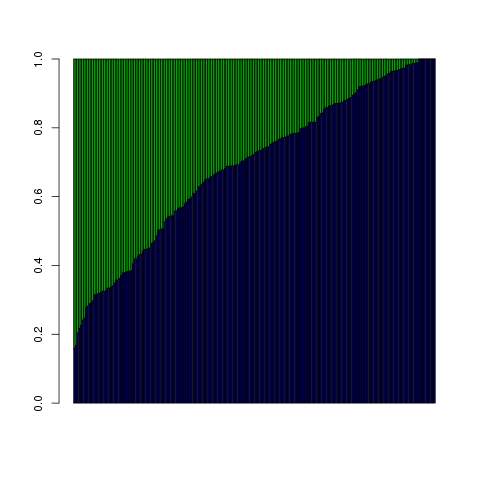
It isn't true for all observations, but it looks like, in aggregate, defense contributions pushed up the probability of voting for continued taps more than ideology did. For some, ideology was entirely irrelevant, but defense contributions had at least a $\sim$ 20% influence for everyone.
So for those cases where we're looking for a large probability, in the typical case it is the defense contributions that make up a bigger chunk of the inputs.
The plot shows a similar pattern for those who voted to defund the wiretap program, with defense contributions dominating even more of the box:
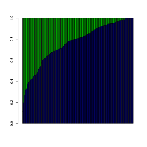
But here, we're looking to explain what would bring about a low probability of supporting the wiretap program, so the fact that defense money was a bigger part of $\beta_0$ + $\beta_1 \cdot \textrm{ideology}$ + $\beta_2 \cdot \textrm{contributions}$ means that it was the bigger push in the wrong direction; the small $\beta_1 \cdot \textrm{ideology}$ is the part that `caused' the final probability to be smaller.
Of course, none of this is about actual causality. We're just looking at an equation that is a sum of components and checking which is bigger or smaller. This is useful, and I think it does tell us something about how to directly compare two things that have different units. That equation fruit = apples + oranges is almost definitional, so all we had to think about was whether we wanted to say that Jane's dearth of oranges on the right-hand side `caused' her dearth of hand fruit on the left-hand side; for vote share the basic equation itself isn't such a clear case.
Elasticity
The Wired article pointed out that those who voted to continue wiretap funding got, on average, twice as much defense funding as those who voted to cut funding.
We can check this from the command line, by reading the data into an on-disk database using Apophenia's standalone text-to-db program, and then using SQLite's standalone program to query the data:
apop_text_to_db amash_vote_analysis.csv atab amash.db
sqlite3 amash.db "select vote, avg(contribs) from atab group by vote"
Output:
Aye  18765.3804878049
No   41635.465437788
Once we round to the nearest dollar, these are exactly the numbers that were printed in Wired's graphic.
But we're not just concerned with total dollars, but with influence within the assumed model. The plots above show the relative influence of contributions to ideology that looks pretty similar for both pro- and anti- sides—certainly not twice as much influence for the yes-tap votes than the no-tap votes.
How much influence did the marginal dollar have? With respect to a known outcome variable, the elasticity of $x$ answers the question: a 1% shift in $x$ leads to what percent of a shift in the outcome? In an equation:
$$E = \frac{\frac{\partial Out}{\partial x}}{\frac{Out}{x}} = \frac{\partial Out}{\partial x}\frac{x}{Out}$$
How does the elasticity of ideology compare to the elasticity of campaign contributions?
The elasticity calculation is one of the computationally nice features of the Logit model, and one of the reasons why people tolerate the clearly false assumptions. If I tell you that the Logit model defines
$$P = \frac{\exp(X\beta)}{1+\exp(X\beta)}$$ (where $X\beta = \beta_0 + X_1 \beta_1 + X_2 \beta_2 + …$) then you could do the math to find that the elasticity for variable $i$ is $$E_i = \frac{X_i\beta_i}{1+\exp(X\beta)}.$$
As with the influence ratios above, the elasticity is different for every observation: people who are at the extreme end of the spectrum are much less responsive to a 1% change in any input than somebody who is on the fence. People who have received no contributions from defense contractors to date may sit up and take notice at the first \$1,000; for many of the congresspeople in our data set, \$1,000 in defense contributions is roundoff.
First the code, then the notes on the code, then the results:
double observation_elasticity(apop_data *in){
    double this_xb = apop_data_get(in, .col=-1);
    double xb = apop_data_get(in, .col=0);
    return  this_xb/(1+exp(xb));
}

apop_data * elasticity(apop_data *d, apop_model *m, char *varname){
    apop_data *xbeta = apop_dot(d, m->parameters);
    Apop_col_t(d, varname, xcol);
    double this_beta=apop_data_get(m->parameters, .rowname=varname);
    gsl_vector_scale(xcol, this_beta);
    xbeta->vector = xcol;
    return apop_map(xbeta, .fn_r=observation_elasticity);
}

//sample use:
apop_data *contribs_elasticity = elasticity(d, logit_out, "contribs");
- Once again, we have a function that will be applied to each row of the data before the main function. An apop_data set has a vector and matrix component, where the vector is treated as the -1th column. I'll have a lot of discussion of that design decision two entries from now; for now, note that putting $X\beta$ in the matrix and $X_i\beta_i$ in the vector gives us all we need to calculate the elasticity.
- So the main function just has to put $X\beta$ in the matrix and $X_i\beta_i$ in the vector. This is easy because the $X$ matrix actually exists in memory in the correct form, so calculating data $\cdot$ params really is apop_dot(d, m->parameters). This is one payoff from having so little subtlety.
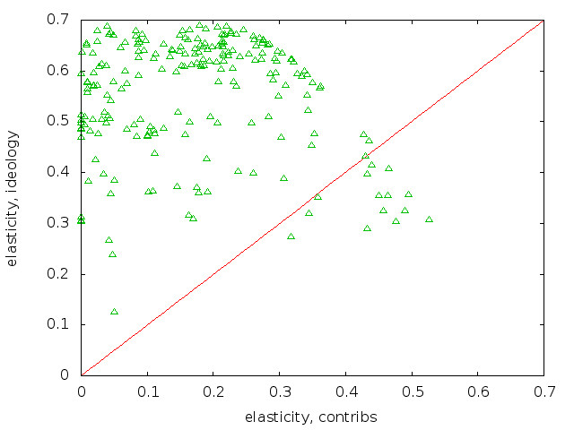
Here are the two elasticity plots, first for the pro-tap voters:
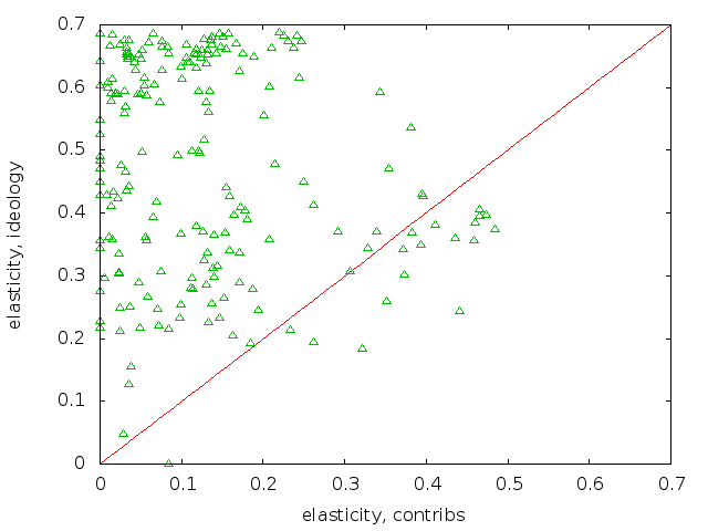
and for the anti-tap voters:
The plots show that the anti-tap voters generally had lower ideology elasticities than those for the pro-tap voters, meaning that a small shift in the anti-tap ideology scores would not have had as much of an effect on their votes. I eyeballed this by opening both plots in a browser tab, then ctrl-tab and ctrl-shift-tabbing between the two tabs. To facilitate this, I fixed the scales to be identical.
I drew in the 1:1 ratio line. Having most of the points above the line, which is the case for both pro- and anti- plots, means that the elasticity from ideology is greater than the elasticity from contributions. In fact, a lot of the contribution elasticities are indistinguishable from zero. That means that if the collected defense industry contributors reduced their collected contribution by \$1, it would have no effect at all. That indicates overspending, but there are a lot of explanations for why this could happen given reasonably rational lobbyists.
For example, contributions are intended to have an effect on may votes, not just this one. This can say a lot about causality: the collected defense contractors chose certain congresspersons to give campaign contributions to, probably based on their potential position on a wide range of defense-related votes. These potential positions are decided by other pre-funding factors, such as ideology, committee memberships, or the ideology of the congressperson's constituent base. We'd need a wider, more narrative model to really explore this broader context.
The conclusion paragraph
As usual, coding the analysis was the easy part. The setup was a series of mechanical manœuvers, the actual model fitting was one line, and the post-analysis was another series of simple operations on matrices. The interesting part is in how the assumptions of the model structure the results. The model implicitly asserts that we can directly compare two terms in the linear combination that goes into calculating the probability. To the extent that you buy that assumption, we can say some things about the relative importance of ideology and contribution terms. The model also asserts a specific equation for elasticity; if we buy the model, then it tells us that the elasticity for the ideology variable is generally larger than the elasticity for campaign contributions. I've already hinted at how, with more data, we could develop other, more descriptive models. But as a first pass, we've already gotten some plausible results about the effect of these two variables on final vote.
Exercise: Dollar amounts are typically treated in log values (e.g., income is typically lognormally distributed), so try all the above using the log of contributions. I used actual dollar amounts because Wired made such a big deal of absolute dollar amounts, but the results are interesting in a different way with log contributions.
[Previous entry: "Do what I mean"]
[Next entry: "Another C macro trick: parenthesized arguments"]